3 The Buckingham \(\Pi\)-theorem and the dimension matrix

Learning outcomes

By the end of this chapter you should be able to:

• state and apply the Buckingham \(\Pi\)-theorem to determine the number of dimensionless groups;

• construct and use the dimension matrix to find the dimensionless complexes systematically;

• interpret the physical meaning of dimensionless groups such as the Reynolds number and the drag coefficient.

3.1 Motivating example: the undamped pendulum

In the previous chapter you met an example of a damped pendulum, we begin this chapter by exploring a simpler problem, the undamped pendulum, in more detail. Consider a simple pendulum: a weight of mass \(m\) suspended from a rigid, massless rod of length \(l\), free to swing in a vertical plane under the influence of gravity. We wish to determine the period of oscillation \(\tau\).

Let \(\theta\) denote the angle between the rod and the downward vertical. Newton’s second law applied to the tangential component of the bob’s motion gives the equation of motion \[m l \ddot{\theta} = -m g \sin\theta,\] where \(g\) is the gravitational acceleration and \(\ddot{\theta} = \dd^2\theta/\dd t^2\). The mass \(m\) cancels immediately, yielding \[\begin{equation} \ddot{\theta} = -\frac{g}{l}\sin\theta. \label{eq:pendulum} \end{equation}\]

This already tells us something important: the motion is independent of the bob’s mass. The governing parameters that remain are \(l\), \(g\) and the initial swing angle, \(\alpha\), (the amplitude). For small oscillations, \(\sin\theta \approx \theta\), and [eq:pendulum] reduces to the equation of simple harmonic motion, \[\ddot{\theta} = -\frac{g}{l}\,\theta,\] whose solution is \(\theta(t) = \alpha \cos(\omega t)\) with angular frequency \(\omega = \sqrt{g/l}\). The period is therefore \[\tau = \frac{2\pi}{\omega} = 2\pi\sqrt{\frac{l}{g}}.\]

We can arrive at essentially the same result (up to the dimensionless numerical prefactor \(2\pi\)) without solving the differential equation at all, using only dimensional considerations. Since \(m\) has cancelled, the period \(\tau\) can depend only on \(l\) and \(g\) (ignoring the angle \(\alpha\) for the moment). The dimensions of these quantities are \[[\tau] = \mathrm{T}, \qquad [l] = \mathrm{L}, \qquad [g] = \mathrm{L\,T}^{-2}.\]

The only combination of \(l\) and \(g\) that has the dimension of time is \(\sqrt{l/g}\): \[\left[\sqrt{\frac{l}{g}}\right] = \left(\frac{\mathrm{L}}{\mathrm{L\,T}^{-2}}\right)^{\!1/2} = \mathrm{T}.\] Hence \(\tau\) must be proportional to \(\sqrt{l/g}\), and we can write \[\tau = C \sqrt{\frac{l}{g}},\] where \(C\) is a dimensionless constant that dimensional analysis alone cannot determine. Comparison with the exact small-angle solution shows that \(C = 2\pi\).

3.2 A systematic method: the dimension matrix

For the pendulum we found the right combination by inspection, because there were only two parameters and a single dimension (time) to match. With more parameters this gu­ess­work quickly becomes hopeless. Fortunately there is a mechanical procedure that always works. We develop it here on the same pendulum problem, so you can see the machinery reproduce an answer you already trust, and then we apply it to harder problems in the worked examples that follow.

The procedure has three practical steps; the third is where the dimension matrix does the work.

Step 1: Identify the governing parameters

This first step requires intuition, common sense, background knowledge and a little creativity. The governing parameters may include:

1. Directly measurable quantities and those to be determined (e.g. the period, length and bob mass of a pendulum).

2. Quantities we believe (or have good reason to consider) important. For the pendulum these might be a friction parameter or the swing angle \(\alpha\). Very often, the list of important parameters emerges gradually, by trial and error.

3. Relevant fundamental constants. For example, include \(g\) or \(G\) if gravity is important, \(\hbar\) to allow for quantum effects, \(c\) (the speed of light) for relativistic effects, and so on.

Pendulum: the governing parameters are \(\tau\), \(l\), \(g\) and \(m\), so \(n = 4\).

Step 2: Count the parameters with independent dimensions

A set of parameters has independent dimensions if none of their dimensions can be built from the dimensions of the others; equivalently, they cannot be combined into a dimensionless quantity. For example, \(l\), \(\tau\) and \(m\) have independent dimensions, but \(l\), \(\tau\) and \(g\) do not, because \[\tau \sqrt{\frac{g}{l}}, \qquad \frac{\tau^{2} g}{l}, \qquad \left(\frac{\tau^{2} g}{l}\right)^{\!p}\] are dimensionless for any power \(p\).

Call the number of parameters with independent dimensions \(k\). It can never exceed the number of basic units in play. In this course the basic units are M (mass), L (length), T (time) and \(\Theta\) (temperature), so \(k\) will not normally exceed four, and is often smaller.

Pendulum: the temperature \(\Theta\) does not appear, so \(k = 3\) (the units M, L and T). If we anticipate that the period cannot depend on the bob’s mass and drop \(m\), then \(k = 2\) (only L and T remain).

The number of independent dimensionless groups we can form is then \[m = n - k.\] For the pendulum, \(m = 4 - 3 = 1\): there is a single dimensionless group to find. (We state this counting rule precisely as the \(\Pi\)-theorem in the next section; for now let us use it.)

Step 3: Build the dimension matrix and solve

Because the dimensions of every parameter are power-law monomials of the basic units, the dimensionless group \(\Pi\) must itself be a power-law monomial of the parameters: \[\begin{equation} \Pi = \tau^{k_1}\, l^{k_2}\, m^{k_3}\, g^{k_4}, \label{eq:Pi-monomial} \end{equation}\] with the exponents \(k_1, k_2, k_3, k_4\) chosen so that \(\Pi\) is dimensionless, \[[\Pi] = 1 = \mathrm{M}^{0}\,\mathrm{L}^{0}\,\mathrm{T}^{0}.\] To find these exponents, write down the dimension matrix, whose columns are the parameters and whose rows are the basic units: \[\begin{array}{c|cccc} & \tau & l & m & g \\ & (k_1) & (k_2) & (k_3) & (k_4) \\ \hline \mathrm{M} & 0 & 0 & 1 & 0 \\ \mathrm{L} & 0 & 1 & 0 & 1 \\ \mathrm{T} & 1 & 0 & 0 & -2 \end{array}\] Each entry is the exponent of that basic unit in the dimension of that parameter. Reading the columns recovers the dimensions we started with: \[[\tau] = \mathrm{T}^{1}, \qquad [l] = \mathrm{L}^{1}, \qquad [m] = \mathrm{M}^{1}, \qquad [g] = \mathrm{L}^{1}\,\mathrm{T}^{-2}.\] Now read the rows. Demanding that the total exponent of each basic unit in [eq:Pi-monomial] vanishes gives one linear equation per row: \[\begin{aligned} \mathrm{M}: &\quad 0\,k_1 + 0\,k_2 + 1\,k_3 + 0\,k_4 = 0, \\ \mathrm{L}: &\quad 0\,k_1 + 1\,k_2 + 0\,k_3 + 1\,k_4 = 0, \\ \mathrm{T}: &\quad 1\,k_1 + 0\,k_2 + 0\,k_3 - 2\,k_4 = 0. \end{aligned}\] These are three equations for four unknowns, one fewer equation than unknown, which is exactly the single degree of freedom (\(m = n - k = 1\)) the counting rule promised. We are therefore free to fix one exponent; since we want a relation of the form \(\tau = F(\ldots)\), take \[k_1 = 1.\] The first equation gives \(k_3 = 0\) (the bob mass does not enter, as expected), and the remaining two reduce to \[k_2 + k_4 = 0, \qquad k_1 - 2k_4 = 0,\] so that \(k_4 = \tfrac{1}{2}\) and \(k_2 = -\tfrac{1}{2}\). Hence \[\Pi = \tau\, l^{-1/2}\, g^{1/2},\] and setting \(\Pi\) equal to a constant recovers \[\boxed{\tau = \Pi \sqrt{\frac{l}{g}},}\] exactly the form we obtained by inspection, now produced by a procedure that will scale to much harder problems.¹

It is worth pausing on what just happened: the \(\Pi\)-theorem is simply the statement that any equation can be rewritten in dimensionless form using units natural to the problem, and it tells us in advance how many dimensionless parameters will appear.

3.3 The \(\Pi\)-theorem (Buckingham’s theorem)

The counting rule we used above has a name and a precise statement.

The reduction from \(n\) parameters to \(m = n - k\) dimensionless ones, even when \(k \le 4\), is an enormous practical saving. To appreciate why, imagine trying to record a relationship as a table of numbers: a function of one variable fits on a single line, a function of two variables fills a page, a function of three variables fills a book, and a function of four variables would fill an entire library.³ Cutting the number of arguments is therefore the difference between a tractable problem and an impossible one.

3.4 Worked example: terminal velocity of a raindrop

A raindrop of mass \(m\) falls through air under gravity until it reaches a constant speed, the terminal velocity \(v\). At terminal velocity the gravitational force is exactly balanced by air resistance, and the drop no longer accelerates. We wish to determine how \(v\) depends on the governing parameters using the dimension matrix.

The relevant governing parameters are:

• \(v\), the terminal velocity;

• \(m\), the mass of the drop;

• \(g\), the gravitational acceleration;

• \(\rho\), the density of air;

• \(A\), the cross-sectional area of the drop.

Step 1. There are \(n = 5\) governing parameters. Their dimensions are: \[[v] = \mathrm{L\,T}^{-1}, \qquad [m] = \mathrm{M}, \qquad [g] = \mathrm{L\,T}^{-2}, \qquad [\rho] = \mathrm{M\,L}^{-3}, \qquad [A] = \mathrm{L}^{2}.\] There are \(k = 3\) base dimensions (M, L, T), so the \(\Pi\)-theorem predicts \(m = n - k = 5 - 3 = 2\) dimensionless groups.

However, we can simplify. At terminal velocity the weight \(mg\) is balanced by drag, so the combination \(mg\) always appears together as a single force. Physically, only the weight \(W = mg\) matters, not \(m\) and \(g\) separately. Replacing them with \(W\) reduces the parameter list to four: \(v\), \(W\), \(\rho\) and \(A\).

Step 2 (revised). Now \(n = 4\) governing parameters with dimensions: \[[v] = \mathrm{L\,T}^{-1}, \qquad [W] = \mathrm{M\,L\,T}^{-2}, \qquad [\rho] = \mathrm{M\,L}^{-3}, \qquad [A] = \mathrm{L}^{2}.\] Still \(k = 3\) base dimensions, so \(m = n - k = 4 - 3 = 1\), a single dimensionless group. The dimension matrix is: \[\begin{array}{c|cccc} & v & W & \rho & A \\ & (k_1) & (k_2) & (k_3) & (k_4) \\ \hline \mathrm{M} & 0 & 1 & 1 & 0 \\ \mathrm{L} & 1 & 1 & -3 & 2 \\ \mathrm{T} & -1 & -2 & 0 & 0 \end{array}\]

Step 3. We seek \(\Pi = v^{k_1}\,W^{k_2}\,\rho^{k_3}\,A^{k_4}\) with \([\Pi] = 1\). The equations for \(k_i\) are: \[\begin{aligned} \mathrm{M}: &\quad k_2 + k_3 = 0, \\ \mathrm{L}: &\quad k_1 + k_2 - 3k_3 + 2k_4 = 0, \\ \mathrm{T}: &\quad -k_1 - 2k_2 = 0. \end{aligned}\] Since we want \(v\) as a function of the other parameters, set \(k_1 = 1\). Then: \[\begin{aligned} \mathrm{T}: &\quad k_2 = -\tfrac{1}{2}k_1 = -\tfrac{1}{2}, \\ \mathrm{M}: &\quad k_3 = -k_2 = \tfrac{1}{2}, \\ \mathrm{L}: &\quad 1 - \tfrac{1}{2} - \tfrac{3}{2} + 2k_4 = 0 \quad\Rightarrow\quad k_4 = \tfrac{1}{2}. \end{aligned}\]

Step 4. The single dimensionless group is: \[\Pi = v\,W^{-1/2}\,\rho^{1/2}\,A^{1/2} = v\sqrt{\frac{\rho A}{W}}.\] Since \(m = 1\), the \(\Pi\)-theorem gives \(\Pi = \text{const}\), i.e. \[\boxed{v = C\sqrt{\frac{W}{\rho A}} = C\sqrt{\frac{mg}{\rho A}},}\] where \(C\) is a dimensionless constant that must be determined experimentally or by solving the full fluid mechanics problem.

3.5 Worked example: drag force on a sphere

We shall now consider a slightly more complicated example which will give rise to two dimensionless complexes rather than one. The drag force \(F_D\) on a sphere depends on its diameter \(L\), velocity \(V\), the fluid density \(\rho\), and the dynamic viscosity \(\mu\). This is the foundation of fluid dynamic similarity.

Step 1: There are \(n = 5\) governing parameters: \(F_D\), \(L\), \(V\), \(\rho\) and \(\mu\). Their dimensions are: \[[F_D] = \mathrm{M\,L\,T}^{-2}, \qquad [L] = \mathrm{L}, \qquad [V] = \mathrm{L\,T}^{-1}, \qquad [\rho] = \mathrm{M\,L}^{-3}, \qquad [\mu] = \mathrm{M\,L}^{-1}\,\mathrm{T}^{-1}.\] There are \(k = 3\) base dimensions: M, L and T. Hence there are \(m = n - k = 5 - 3 = 2\) dimensionless complexes.

Step 2: The dimension matrix has the form \[\begin{array}{c|ccccc} & F_D & L & V & \rho & \mu \\ & (k_1) & (k_2) & (k_3) & (k_4) & (k_5) \\ \hline \mathrm{M} & 1 & 0 & 0 & 1 & 1 \\ \mathrm{L} & 1 & 1 & 1 & -3 & -1 \\ \mathrm{T} & -2 & 0 & -1 & 0 & -1 \end{array}\] and we seek \(\Pi = F_D^{k_1}\,L^{k_2}\,V^{k_3}\,\rho^{k_4}\,\mu^{k_5}\) with \([\Pi] = 1\). The equations for \(k_i\) follow as \[\begin{aligned} \mathrm{M}: &\quad k_1 + k_4 + k_5 = 0, \\ \mathrm{L}: &\quad k_1 + k_2 + k_3 - 3k_4 - k_5 = 0, \\ \mathrm{T}: &\quad -2k_1 - k_3 - k_5 = 0, \end{aligned}\] three equations for five unknowns. Since \(m = 2\), two of the exponents can be chosen freely.

Step 3: first \(\Pi\)-group. Put \(k_1 = 1\) and \(k_5 = 0\). Then \[\begin{aligned} \mathrm{M}: &\quad k_4 = -k_1 = -1, \\ \mathrm{T}: &\quad k_3 = -2k_1 = -2, \\ \mathrm{L}: &\quad 1 + k_2 - 2 + 3 = 0 \quad\Rightarrow\quad k_2 = -2, \end{aligned}\] which gives the first dimensionless complex: \[\Pi_1 = \frac{F_D}{\rho\,V^{2}\,L^{2}}.\] This is recognised as the drag coefficient \(C_D\) (up to a conventional numerical factor).

Step 4: second \(\Pi\)-group. Put \(k_1 = 0\) and \(k_5 = 1\). Then \[\begin{aligned} \mathrm{M}: &\quad k_4 = -k_5 = -1, \\ \mathrm{T}: &\quad k_3 = -k_5 = -1, \\ \mathrm{L}: &\quad k_2 - 1 + 3 - 1 = 0 \quad\Rightarrow\quad k_2 = -1, \end{aligned}\] which gives the second dimensionless complex: \[\Pi_2 = \frac{\mu}{\rho\,V\,L}.\] The reciprocal of \(\Pi_2\) is the Reynolds number, \(\mathrm{Re} = \rho V L / \mu\).

Result. The \(\Pi\)-theorem tells us that \[\boxed{\Phi(\Pi_1, \Pi_2) = 0, \qquad \text{or equivalently} \qquad C_D = C_D(\mathrm{Re}).}\]

Worked example: the Sedov–Taylor blast wave

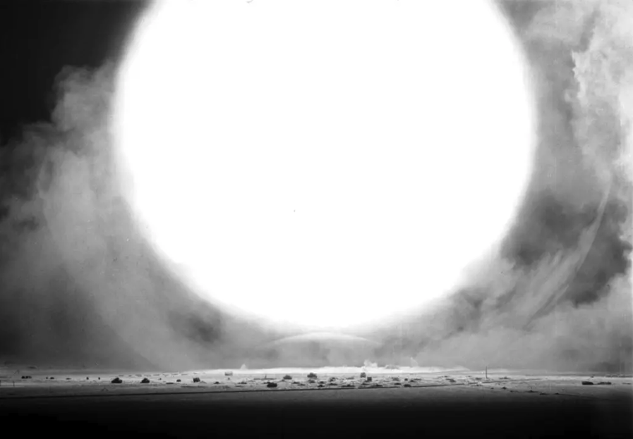
A nuclear explosion can be considered with an appropriate and reasonable idealisation as an instantaneous release of a certain energy, \(E\), which causes an expanding shock wave to propagate outwards. As the amount of energy released is very large, pressure inside the expanding, very hot region is by far larger than that in the surrounding medium, say, air. This leads to a rapid expansion of the hot gas region, the fireball. Since the expansion is so fast, the gas energy lost during the expansion at this early stage is negligible, so \(E = \text{const}\) is a good approximation at early stages of the expansion, where \(E\) is the total energy of the fireball. Obviously, this energy is very close to the energy released in the explosion: the original air energy within the heated region is negligible in comparison with the explosion energy. However, the ambient gas mass density \(\rho\) cannot be neglected because the mass of the gas produced in the explosion (the explosion debris) is negligible and the hot air is largely the ambient air heated by the radiation produced in the explosion and swept up by the outer boundary of the expanding hot region.

Apart from \(E\) and \(\rho\), the governing parameters of the problem are \(t\), time elapsed after the energy release, and \(R\), the size of the hot region.

At an early stage after the energy release the hot region expands so rapidly that, when the lower part of it encounters the Earth surface (if the explosion charge is located on top of a tower or is dropped from an airplane and explodes in air), the upper part is not affected and remains spherical for a relatively long time. Thus, it is not unreasonable to assume that the expanding hot region is spherically symmetric, hence it is called a fireball.

Applying the dimension matrix. The governing parameters and their dimensions are: \[[E] = \mathrm{M\,L}^{2}\,\mathrm{T}^{-2}, \qquad [\rho] = \mathrm{M\,L}^{-3}, \qquad [t] = \mathrm{T}, \qquad [R] = \mathrm{L},\] and our goal is to find how \(R\) depends on the other parameters. The dimension matrix has the form \[\begin{array}{c|cccc} & E & \rho & t & R \\ & (k_1) & (k_2) & (k_3) & (k_4) \\ \hline \mathrm{M} & 1 & 1 & 0 & 0 \\ \mathrm{L} & 2 & -3 & 0 & 1 \\ \mathrm{T} & -2 & 0 & 1 & 0 \end{array}\] and equations for \(k_i\) follow as \[\begin{aligned} \mathrm{M}: &\quad k_1 + k_2 = 0, \\ \mathrm{L}: &\quad 2k_1 - 3k_2 + k_4 = 0, \\ \mathrm{T}: &\quad -2k_1 + k_3 = 0, \end{aligned}\] and we put \(k_4 = 1\). This leads to \[\begin{aligned} \mathrm{M}: &\quad k_2 = -k_1, \\ \mathrm{L}: &\quad 2k_1 - 3k_2 + 1 = 0, \\ \mathrm{T}: &\quad k_3 = 2k_1, \end{aligned}\] which solves to yield \[k_1 = -\tfrac{1}{5}, \qquad k_2 = \tfrac{1}{5}, \qquad k_3 = -\tfrac{2}{5}.\] We have thus derived the following dimensionless complex of the governing parameters: \[\Pi = E^{-1/5}\,\rho^{1/5}\,t^{-2/5}\,R,\] which leads to the desired result: \[\begin{equation} \boxed{R = \Pi\left(\frac{Et^{2}}{\rho}\right)^{\!1/5}.} \label{eq:sedov-taylor} \end{equation}\]

This is the famous expansion law of an explosion fireball known as the Sedov–Taylor solution. It was first derived in 1941 by Geoffrey Ingram Taylor (1886–1975) in the UK, John von Neumann (1903–1957) in the USA and Leonid Ivanovich Sedov (1907–1999) in the USSR (published in 1946, but derived earlier).

In 1950, Sir Geoffrey Taylor published a paper where he analysed photographs of the first atomic explosion in New Mexico declassified in 1947. Sir Geoffrey found that the expansion of the fireball was described by [eq:sedov-taylor] to an impressive degree of accuracy, and obtained, from fitting it to the observed expansion, the explosion energy \(E\). This paper caused a scandal in the USA military and intelligence establishment since, unlike the photographs of the explosion, the charge energy remained highly classified.

This solution also describes explosions of another kind and scale, explosions of young, hot, massive, rapidly evolving stars, leading to the appearance of extremely bright supernova stars. The supernova of 1054 AD was, at its peak, brighter than any star or planet in the sky and remained visible in daylight for over three weeks; it was recorded in historical chronicles around the world (the supernova exploded some 6,500 light years away). Its remnant is now known as the Crab nebula.

Supernova explosions drive the turbulence in the interstellar gas whose scale is close to the size of the fireball at a time when its expansion speed \(\dd R/\dd t\) becomes comparable to the speed of sound in the ambient gas, at the early stages of supersonic expansion no perturbation can propagate ahead of the shock, except for light.