By the end of this chapter you should be able to:
identify characteristic scales in a physical problem;
nondimensionalise a first-order ODE by introducing dimensionless variables;
interpret the resulting dimensionless parameters;
explain why nondimensional solutions are universal (solution collapse).
Key Idea
What do we mean by scaling? To scale a quantity is to measure it against a reference value that is natural for the problem, instead of in everyday units such as seconds or kelvin. We choose a reference value, called a scale, and divide by it: \[\text{scaled quantity} = \frac{\text{quantity}}{\text{its scale}}.\] You already do this every day. Your phone shows its battery as a percentage rather than as an amount of charge: it divides the charge left by the full capacity. So \(50\%\) means “half full” on any phone, however big its battery.
A scaled quantity has no units, because the units cancel in the division. It tells you straight away whether the quantity is large or small for this problem. For Newton’s cooling example below, dividing the temperature excess by its starting value gives \[\theta = \frac{T - T_\infty}{T_0 - T_\infty},\] which is \(1\) at the start, \(\tfrac12\) when the object has lost half its excess heat, and \(0\) when it reaches room temperature. This is true whatever the starting temperature, and whether you measure in kelvin or degrees Celsius. Time can be scaled in the same way, by measuring it in units of the natural cooling time \(1/k\). So \(s = kt = 1\) means “one cooling time has passed”.
Scaling does not change the model. It only changes the units we measure in, from human units (seconds, kelvin) to the problem’s own units. Section 2.1 shows how to choose the scales, and Sections 2.2–2.3 show how to rewrite an equation in scaled variables.
When we write down a model, the variables and parameters carry units. For instance, in Newton’s cooling law \[\ddt{T} = -k(T - T_{\infty}),\] the temperature \(T\) is in kelvin, \(t\) in seconds, \(k\) in \(\mathrm{s}^{-1}\), and \(T_\infty\) is a reference temperature.
A characteristic scale is a representative value of a quantity that captures the natural “size” of that quantity in the problem. Common choices:
For temperature excess: \(T_0 - T_\infty\), the initial excess above ambient.
For time: \(1/k\), the natural relaxation time.
For length: the size of the domain or a physical feature.
The idea is to make variables dimensionless by dividing by their characteristic scale. This removes units and reduces the number of parameters.
The strategy is: identify the dimensional variables and parameters, choose a representative scale for each variable, define dimensionless variables by dividing, and rewrite the equation. The dimensionless groups that survive the rescaling are the ones that genuinely govern the behaviour. The worked example below makes each step concrete.
Consider again \[\ddt{T} = -k(T - T_\infty), \qquad T(0) = T_0.\]
Step 1. Dimensional variables: \(T\) (temperature, K), \(t\) (time, s). Parameters: \(k\ [\mathrm{s}^{-1}]\), \(T_\infty\ [\mathrm{K}]\), \(T_0\ [\mathrm{K}]\).
Step 2. Characteristic scales: temperature scale \(\Delta T = T_0 - T_\infty\), time scale \(\tau = 1/k\).
Step 3. Define \[\theta = \frac{T - T_\infty}{T_0 - T_\infty}, \qquad s = k\,t.\] Both \(\theta\) and \(s\) are dimensionless.
Step 4. Rewrite the ODE in the new variables. First write the old variables in terms of the new ones, by rearranging the definitions in Step 3: \[T = T_\infty + (T_0 - T_\infty)\,\theta, \qquad t = \frac{s}{k}.\] The ODE contains \(\dd T/\dd t\), but our unknown is now \(\theta\) as a function of \(s\). Since \(T\) depends on \(s\), and \(s\) depends on \(t\), the chain rule gives \[\frac{\dd T}{\dd t} = \frac{\dd T}{\dd s}\cdot\frac{\dd s}{\dd t}.\] We work out each factor separately.
\(T_\infty\) and \(T_0 - T_\infty\) are constants, so differentiating \(T = T_\infty + (T_0 - T_\infty)\theta\) with respect to \(s\) gives \(\dfrac{\dd T}{\dd s} = (T_0 - T_\infty)\dfrac{\dd\theta}{\dd s}\).
\(s = kt\) with \(k\) constant, so \(\dfrac{\dd s}{\dd t} = k\).
Multiplying the two factors, \[\frac{\dd T}{\dd t} = k\,(T_0 - T_\infty)\,\frac{\dd\theta}{\dd s}.\] On the right-hand side of the ODE, \(T - T_\infty = (T_0 - T_\infty)\theta\). Substituting both into \(\dd T/\dd t = -k(T - T_\infty)\): \[k\,(T_0 - T_\infty)\,\frac{\dd\theta}{\dd s} = -k\,(T_0 - T_\infty)\,\theta.\]
Step 5. Divide through by \(k(T_0 - T_\infty)\), the coefficient of the derivative, so that the derivative stands alone. Finally convert the initial condition: at \(t = 0\) we have \(s = 0\) and \(T = T_0\), so \(\theta(0) = (T_0 - T_\infty)/(T_0 - T_\infty) = 1\). This gives \[\boxed{\frac{\dd\theta}{\dd s} = -\theta, \qquad \theta(0) = 1.}\]
This is a universal equation — it contains no parameters at all. Its solution is simply \[\theta(s) = e^{-s}.\]
Key Idea
By choosing the right scales, we have removed all parameters. Every Newton’s cooling problem — regardless of \(k\), \(T_0\), \(T_\infty\) — maps to the same dimensionless solution \(\theta = e^{-s}\). This is solution collapse.
To visualise collapse: suppose you solve the dimensional problem for three different values of \(k\) (say 0.1, 0.5, and 2.0 s\(^{-1}\)) and plot \(T(t)\) vs \(t\). You get three distinct curves.
Now plot \(\theta(s) = (T - T_\infty)/(T_0 - T_\infty)\) vs \(s = kt\) for all three. All three curves coincide exactly on \(e^{-s}\). This is the power of nondimensionalisation.
Example: Logistic growth — nondimensionalisation preview
The logistic equation is \[\ddt{N} = r\,N\!\left(1 - \frac{N}{K}\right), \qquad N(0) = N_0.\] Let \(u = N/K\) (dimensionless population) and \(s = rt\) (dimensionless time). Show that \[\frac{\dd u}{\dd s} = u(1-u), \qquad u(0) = N_0/K.\] The original three parameters \((r, K, N_0)\) reduce to just one: \(N_0/K\).
When nondimensionalising a more complicated equation, not all parameters always cancel. What remains are dimensionless groups — combinations of the original parameters that have no units.
These groups carry physical meaning. For instance:
The Reynolds number \(Re = \rho U L / \mu\) in fluid mechanics compares inertial to viscous forces.
The Damköhler number \(Da\) in chemistry compares reaction to diffusion timescales.
A single dimensionless group governs the qualitative behaviour of the solution. Next week we will see a systematic method — the Buckingham \(\Pi\) theorem — for finding these groups from the dimensional parameters alone.
Exercise 2.1
The equation for a damped pendulum is \[m L^2\,\ddot\theta + b L^2\,\dot\theta + mg L\,\sin\theta = 0.\]
Identify all dimensional quantities and their dimensions.
Choose characteristic scales for angle and time.
Show that nondimensionalisation leads to \[\ddot u + \gamma\,\dot u + \sin u = 0,\] where \(\gamma = \dfrac{b}{m}\sqrt{\dfrac{L}{g}}\) is the only dimensionless parameter. State clearly what \(\gamma\) measures physically.
Exercise 2.2
A chemical concentration \(C\) evolves as \[\frac{\dd C}{\dd t} = -\frac{C}{\tau_r} + S,\] where \(\tau_r\) is a reaction timescale and \(S\) is a constant source.
Nondimensionalise using \(C^* = C/(S\tau_r)\) and \(s = t/\tau_r\).
What is the steady state of the nondimensional equation?
What does this tell you about the original dimensional steady state?
This section takes one everyday example through the main ideas of Chapters 1 and 2: building a model, checking its dimensions, solving it, and then nondimensionalising it step by step. If you are comfortable with Sections 2.1–2.4, you can skip it, once you’re happy with this example you’ve got the key ideas of the modelling aspects of the course.
You have \(B_0 = \textup{\pounds}10{,}000\) in a savings account that pays interest of \(0.5\%\) per month, and you withdraw \(W = \textup{\pounds}500\) per month. How long will the money last? A quick answer is \(10{,}000/500 = 20\) months, but the interest should make it last a little longer.
Formulate (Section 1.6). Let \(B(t)\) be the balance, in pounds, at time \(t\), in months. We assume interest is added continuously and withdrawals are spread evenly, and that nothing else happens. The word equation is \[\text{rate of change of balance} = \text{interest coming in} - \text{withdrawals going out}.\] Interest is proportional to the balance (twice the money earns twice the interest), so it comes in at rate \(rB\), where \(r = 0.005\) per month. Withdrawals go out at the constant rate \(W\). So \[\boxed{\ddt{B} = rB - W, \qquad B(0) = B_0.}\] With \(W = 0\) this is the exponential growth model of Section 1.4.
Check dimensions (Section 1.3). Money is not mass, length or time, so we give it its own base dimension, written \(\textup{\pounds}\), just as temperature has its own dimension \(\Theta\). Then \([B] = [B_0] = \textup{\pounds}\), \([t] = \mathrm{T}\), \([r] = \mathrm{T}^{-1}\) and \([W] = \textup{\pounds}\,\mathrm{T}^{-1}\). Every term in the ODE has the same dimensions: \[\left[\ddt{B}\right] = \frac{[B]}{[t]} = \textup{\pounds}\,\mathrm{T}^{-1}, \qquad [rB] = \mathrm{T}^{-1}\cdot\textup{\pounds} = \textup{\pounds}\,\mathrm{T}^{-1}, \qquad [W] = \textup{\pounds}\,\mathrm{T}^{-1}. \quad\checkmark\]
Solve (Section 1.4.2). Factor out \(r\), separate the variables and integrate: \[\ddt{B} = r\left(B - \frac{W}{r}\right) \quad\Longrightarrow\quad \int\frac{\dd B}{B - W/r} = \int r\,\dd t,\] and since \(W/r\) is a constant, \[\log\left|B - \frac{W}{r}\right| = rt + c.\] Taking exponentials, \(B - W/r = Ae^{rt}\) with \(A = \pm e^{c}\), and \(B(0) = B_0\) gives \(A = B_0 - W/r\). So \[B(t) = \frac{W}{r} + \left(B_0 - \frac{W}{r}\right)e^{rt}.\] The equilibrium is \(B^{*} = W/r = \textup{\pounds}100{,}000\): the balance at which interest exactly pays for the withdrawals. Starting below it, the balance falls until it reaches zero. Setting \(B = 0\) and solving for \(t\) gives \[t^{*} = \frac{1}{r}\log\left(\frac{W}{W - rB_0}\right) = 200\log\left(\frac{500}{450}\right) \approx 21.1 \text{ months}.\] Interest adds about a month.
We now follow the five steps of Section 2.3, writing out every line.
Step 1. The variables are \(B\) (dimensions \(\textup{\pounds}\)) and \(t\) (dimensions \(\mathrm{T}\)). The parameters are \(r\) (\(\mathrm{T}^{-1}\)), \(W\) (\(\textup{\pounds}\,\mathrm{T}^{-1}\)) and \(B_0\) (\(\textup{\pounds}\)).
Step 2. We need a scale for money and a scale for time, each built from the parameters and with the right dimensions. For money, the natural choice is the starting balance \(B_0\). For time, since \([r] = \mathrm{T}^{-1}\), the simplest choice is \(1/r = 200\) months: the time scale on which interest acts.
Step 3. Divide each variable by its scale: \[b = \frac{B}{B_0}, \qquad s = \frac{t}{1/r} = rt.\] Both are pure numbers: \([b] = \textup{\pounds}/\textup{\pounds} = 1\) and \([s] = \mathrm{T}^{-1}\cdot\mathrm{T} = 1\). So \(b\) is the balance as a fraction of what you started with, and \(s\) is time measured in units of \(1/r\).
Step 4. Rewrite the ODE in the new variables. First write the old variables in terms of the new ones: \[B = B_0\,b, \qquad t = \frac{s}{r}.\] The ODE contains \(\dd B/\dd t\), but our unknown is now \(b\) as a function of \(s\).
Key Idea
Rates depend on your clock. If your balance falls by \(\textup{\pounds}500\) per month, it falls by \(\textup{\pounds}6000\) per year, because \[\frac{\text{change}}{\text{year}} = \frac{\text{change}}{\text{month}}\times\frac{\text{months}}{\text{year}}.\] Changing from \(t\) to \(s\) is changing to a new clock, and the chain rule is the same calculation written with derivatives.
Since \(B\) depends on \(s\), and \(s\) depends on \(t\), the chain rule gives \[\ddt{B} = \frac{\dd B}{\dd s}\cdot\frac{\dd s}{\dd t}.\] We work out each factor separately.
\(B = B_0\,b\) with \(B_0\) constant, so \(\dfrac{\dd B}{\dd s} = B_0\dfrac{\dd b}{\dd s}\).
\(s = rt\) with \(r\) constant, so \(\dfrac{\dd s}{\dd t} = r\).
Multiplying the two factors, \[\ddt{B} = rB_0\,\frac{\dd b}{\dd s}.\] Now substitute this, and \(B = B_0 b\), into \(\dd B/\dd t = rB - W\): \[rB_0\,\frac{\dd b}{\dd s} = r\,B_0\,b - W.\]
Step 5. Divide through by \(rB_0\), the coefficient of the derivative: \[\frac{\dd b}{\dd s} = b - \frac{W}{rB_0}.\] One combination of parameters is left over. Call it \[\alpha = \frac{W}{rB_0}, \qquad\text{and check:}\qquad [\alpha] = \frac{\textup{\pounds}\,\mathrm{T}^{-1}}{\mathrm{T}^{-1}\cdot\pounds} = 1,\] so \(\alpha\) is a dimensionless group. Finally convert the initial condition: at \(t = 0\) we have \(s = 0\) and \(B = B_0\), so \(b(0) = 1\). The whole problem is now \[\boxed{\frac{\dd b}{\dd s} = b - \alpha, \qquad b(0) = 1.}\] Three parameters (\(B_0\), \(r\), \(W\)) have become one (\(\alpha\)).
Common mistakes.
Forgetting the factor \(\dd s/\dd t\) from the chain rule, and writing \(\dd B/\dd t = B_0\,\dd b/\dd s\) without the \(r\). This is the most common error.
Forgetting to convert the initial condition.
Choosing a “scale” with the wrong dimensions. Check every scale before you use it.
The group has a clear meaning: \[\alpha = \frac{W}{rB_0} = \frac{\text{rate of spending}}{\text{rate of earning interest at the start}}.\] For our example, \(\alpha = 500/(0.005 \times 10{,}000) = 500/50 = 10\): you spend ten times faster than interest comes in. Working in years instead (\(W = 6000\) per year, \(r = 0.06\) per year) gives \(\alpha = 6000/600 = 10\) again. A dimensionless group does not depend on the units you choose.
The dimensionless problem is the original one with \(r = 1\), \(W = \alpha\) and \(B_0 = 1\), so its solution is \(b(s) = \alpha + (1 - \alpha)e^{s}\). The single number \(\alpha\) decides the behaviour: if \(\alpha < 1\) the balance grows for ever; if \(\alpha = 1\) it stays constant; and if \(\alpha > 1\) the money runs out, at \(s^{*} = \log\bigl(\alpha/(\alpha - 1)\bigr)\).
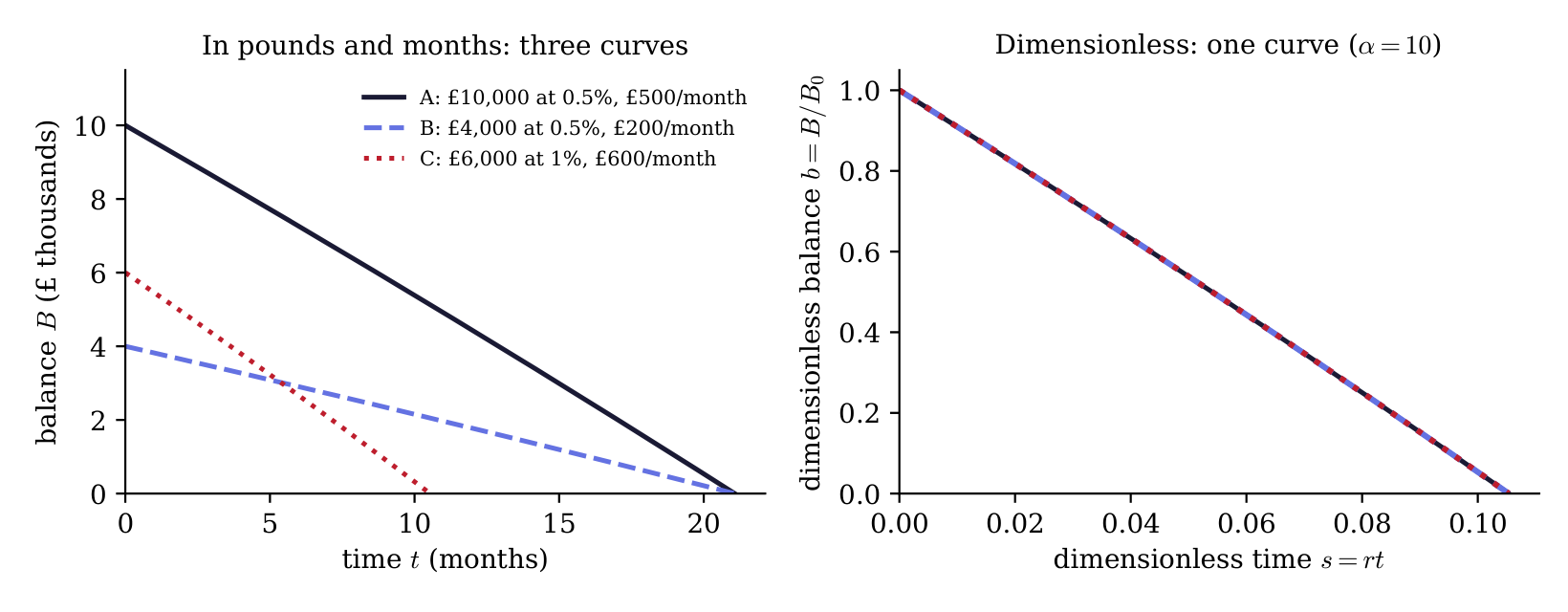
Accounts with very different \(B_0\), \(r\) and \(W\) behave identically if they share the same value of \(\alpha\). For example, these three accounts all have \(\alpha = 10\):
| Account | \(B_0\) | \(r\) (per month) | \(W\) (per month) | money lasts |
|---|---|---|---|---|
| A | £10,000 | \(0.5\%\) | £500 | 21.1 months |
| B | £4,000 | \(0.5\%\) | £200 | 21.1 months |
| C | £6,000 | \(1\%\) | £600 | 10.5 months |
Plotted in pounds and months they give three different curves, but plotted as \(b\) against \(s\) they lie exactly on top of one another (Figure 2.1).
Key Idea
Nondimensionalising replaced a three-parameter family of answers with a one-parameter family, and the remaining parameter has a clear meaning. Accounts with the same \(\alpha\) collapse onto the same curve. This is exactly what happened for Newton’s cooling in Section 2.4, where no parameters survived at all.
Checklist for nondimensionalising a first-order ODE.
List the variables and parameters, with their dimensions.
Choose a scale for each variable, built from the parameters, with the same dimensions as the variable.
Define dimensionless variables by dividing each variable by its scale.
Write the old variables in terms of the new ones, convert the derivative with the chain rule (including the factor \(\dd s/\dd t\)), and substitute.
Divide by the coefficient of the derivative, name any leftover groups and check they are dimensionless, and convert the initial condition.